How to define an evaluation task

This notebook demonstrates how bobbin can help building evaluation.

Preamble: Install prerequisites, import modules.

!pip -q install --upgrade pip
!pip -q install --upgrade "jax[cpu]"
!pip -q uninstall -y bobbin
!pip -q install --upgrade git+https://github.com/yotarok/bobbin.git

%%capture
from typing import Tuple

import bobbin
import chex
import flax
import flax.linen as nn
import jax
import jax.numpy as jnp
import numpy as np
import optax
import tensorflow_datasets as tfds
import matplotlib.pyplot as plt

chex.set_n_cpu_devices(8)

Array = chex.Array

Prepare a model to be evaluated

First, we train a small model to be evaluated over the MNIST datasets. For more details in training with bobbin, please refer How to write a training loop.

The function below is a definition for dataset pipelines.

def get_dataset(batch_size, *, is_train=True, split="train"):
    ds = tfds.load("mnist", split=split, as_supervised=True)
    if is_train:
        ds = ds.repeat().shuffle(1024)
    ds = ds.batch(batch_size).prefetch(1)
    return ds

Note that the dataset is infinite only when is_train == True.

Here, a simple linear classifier is defined as a Flax module, also bobbin.TrainTask subclass is implemented for defining cross-entropy trainng over that simple classifier. (See training doc for details.)

class MnistLinearClassifier(nn.Module):
    @nn.compact
    def __call__(self, x: Array) -> Array:
        batch_size, *unused_image_dims = x.shape
        x = x.reshape((batch_size, -1))  # flatten the input image.
        return nn.Dense(features=10)(x)


class MnistTrainingTask(bobbin.TrainTask):
    def __init__(self):
        super().__init__(
            MnistLinearClassifier(),
            example_args=(
                np.zeros((1, 28, 28, 1), np.float32),  # comma-here is important
            ),
        )

    def compute_loss(self, params, batch, *, extra_vars, prng_key, step):
        images, labels = batch
        logits = self.model.apply({"params": params}, images)
        per_sample_loss = optax.softmax_cross_entropy(
            logits=logits, labels=jax.nn.one_hot(labels, 10)
        )
        return jnp.mean(per_sample_loss), ({}, None)


task = MnistTrainingTask()
train_state = task.initialize_train_state(
    jax.random.PRNGKey(0), optax.sgd(0.001, momentum=0.9)
)
train_step_fn = task.make_training_step_fn()

No GPU/TPU found, falling back to CPU. (Set TF_CPP_MIN_LOG_LEVEL=0 and rerun for more info.)

500 steps of stochastic gradient descent are done as follows:

prng_key = jax.random.PRNGKey(0)
for batch in get_dataset(64).take(500).as_numpy_iterator():
    rng, prng_key = jax.random.split(prng_key)
    train_state, step_info = train_step_fn(train_state, batch, rng)
print(f"Last loss value = {step_info.loss}")

Last loss value = 34.819725036621094

Define EvalResults

First, we define the metric used for evaluation. Here, also for demonstrating SampledSet, the result is containing both confusion matrices and sampled triples of inputs, outputs, and labels.

class EvalResults(bobbin.EvalResults):
    confusion_matrix: Array
    examples: bobbin.SampledSet[Tuple[int, int, Array]] = flax.struct.field(
        pytree_node=False, default=bobbin.SampledSet(max_size=4)
    )
    dataset_name: str = flax.struct.field(pytree_node=False, default="")

    def prediction_count(self) -> int:
        return jnp.sum(self.confusion_matrix)

    def correct_count(self) -> int:
        return jnp.sum(jnp.diag(self.confusion_matrix))

    def accuracy(self) -> float:
        return self.correct_count() / self.prediction_count()

    def reduce(self, other: "EvalResults") -> "EvalResults":
        return type(self)(
            confusion_matrix=self.confusion_matrix + other.confusion_matrix,
            examples=self.examples.union(other.examples),
        )

EvalResults is a subclass of flax.dataclass.PyTreeNode that means that it follows Python’s dataclass semantics. The type annotations at the beginning of the class definition are also used as a list of fields, and some special methods, e.g. constructors, are created automatically according to the list of fields.

Here, it should be noted that some of fields (“examples” and “dataset_name” in this example) are explicitly excluded from pytree definition by setting pytree_node=False. This is especially important when we do use JIT-ed function in the EvalTask below. Anything that is passed to the compiled (JIT-ed) function must have a jax representation, and some types like str doesn’t have that. Therefore, we have to exclude those things from pytree so they are treated as non-jax variables.

A subclass of bobbin.EvalTask is defined for implementing how to compute EvalResults above.

class EvalTask(bobbin.EvalTask):
    def __init__(self):
        self.model = MnistLinearClassifier()

    def create_eval_results(self, dataset_name):
        return EvalResults(
            confusion_matrix=np.zeros((10, 10)),
            examples=bobbin.SampledSet(max_size=4),
            dataset_name=dataset_name,
        )

    def evaluate(self, batch, model_vars) -> EvalResults:
        inputs, labels = batch
        logits = self.model.apply(model_vars, inputs)
        predicts = logits.argmax(axis=-1)
        confusion_mat = jnp.dot(
            jax.nn.one_hot(predicts, 10).T, jax.nn.one_hot(labels, 10)
        )
        examples = bobbin.SampledSet(max_size=4).union(
            zip(predicts, labels, list(inputs))
        )
        return EvalResults(confusion_matrix=confusion_mat, examples=examples)

EvalTask.create_eval_results is used for initializing the EvalResults instance. For each incoming batch, EvalTask.evaluate is called, and the results are combined following the pseudo-code below:

result = eval_task.create_eval_results(...)
for b in batches:
    result = result.reduce(eval_task.evaluate(b, ...))

The datasets given to the evaluation process are represented as a (nullary) function that returns iterator of batches. If we use tf.data API for representing the dataset, we can easily obtain such function as follows:

eval_datasets = {
    "train": get_dataset(32, split="train[:1000]", is_train=False).as_numpy_iterator,
    "test": get_dataset(32, split="test", is_train=False).as_numpy_iterator,
}

Actual computation can be invoked by calling bobbin.eval_datasets as below. (The function below basically just performs the for-loop based implementation written in the pseudo-code above, so you may write it down on your codebase.)

eval_task = EvalTask()
all_results = bobbin.eval_datasets(
    eval_task, eval_datasets, {"params": train_state.params}
)
all_results.keys()

dict_keys(['train', 'test'])

Here, you obtained all_results: dict[str, EvalResults] containing accumulated results for each dataset given. You can compute accuracies over the results, and also visualize the confusion matrix, as follows:

for dataset_name, results in all_results.items():
    print(f"dataset={dataset_name}:\tAccuracy = {results.accuracy()}")

plt.subplot(1, 2, 1)
plt.imshow(all_results["train"].confusion_matrix)
plt.title("train")
plt.subplot(1, 2, 2)
plt.imshow(all_results["test"].confusion_matrix)
plt.title("test")

dataset=train:	Accuracy = 0.847000002861023
dataset=test:	Accuracy = 0.8457000255584717

Text(0.5, 1.0, 'test')

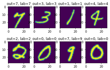
EvalResults.examples field holds 4 random samples of input-label-output triples. Here, we can visualize how classifier worked as follows:

index = 1
for pred, lab, inputs in all_results["train"].examples:
    plt.subplot(2, 4, index)
    plt.imshow(inputs.reshape((28, 28)))
    plt.title(f"out={pred}, lab={lab}")
    index += 1
for pred, lab, inputs in all_results["test"].examples:
    plt.subplot(2, 4, index)
    plt.imshow(inputs.reshape((28, 28)))
    plt.title(f"out={pred}, lab={lab}")
    index += 1